Main menu
You are here
Applying An Epidemiological Model
As those of you who read my third most recent post will know, I recently became excited about methods for predicting the spread of diseases mathematically. When I learned about compartmental models, I began searching for tips on how they could best be applied to real data. I stumbled upon a solution on Abraham Flaxman's blog, Healthy Algorithms.
In Abraham's post, he presents some code that will estimate the parameters in a dynamical system using Bayesian Inference - the most elegant thing to come out of statistics since the Central Limit Theorem. Also present is an exercise challenging the reader to estimate the parameters of a 1967 smallpox outbreak in Nigeria.
If you want to do this exercise without a spoiler then stop! Otherwise, keep reading and I will tell you how I approached the problem while making some random remarks on the strengths and weaknesses of this particular fitting routine.
Following the suggestions, we will use the SEIR model to analyse the smallpox outbreak. This means that people can contract the disease without infecting others right away. For simplicity, we will consider the discrete version of this model. So instead of differential equations, we will write down the analogous difference equations:
 |
Next, we have to decide what data we actually have. To demonstrate the method, Abraham estimates the parameters of an SIR model assuming that values of  and
and  are known at particular times. In reality, it is often impossible to find this type of data. Why don't we know ? Well it is hard to agree on what makes someone "susceptible" when a disease affects a population. If cases of a disease start showing up in a certain city some people might say that the number of susceptible people is initially the population of the city. But sometimes there is really only one neighbourhood where the epidemic originates and it just takes people a long time to find the source of it. On the other hand, the susceptible population sometimes extends beyond the city where an epidemic is first discovered. People who live in the surrounding suburbs certainly have some risk of being infected. And if enough people travel, it might be the entire country that one considers susceptible.
Why don't we know ? I think this is simply because hospitals are busy. If many sick people are showing up at a hospital every day and that hospital is required to report statistics to the Ministry of Health, it makes sense to say "on day one we got 7 new patients, on day two we got 12 and on day three we got 11" in the report. To report the number of infected individuals on a given day, the staff would have to visit the hospital room of every person that they have ever seen infected and check each person to see if he or she has recovered yet. Even though the 1967 outbreak we're dealing with only produced 33 cases, the WHO still did not report  as a time series. This might be because some privacy policy forbids it. Have you seen these types of disclaimers?
All participants are anonymous. Furthermore, information gathered will be aggregate and will not be associated with a specific individual. No individual will be identifiable from any publications arising from this reasearch.
I know I have (when I fill out such a survey I usually include a note waiving my right to anonymity hoping that it will allow the researcher to do a better job). Maybe this is what makes the number of newly infected people a more common statistic than the number of currently infected people.
In any case, we know how many new people became infected (developed a visible rash) from one day to the next because the WHO report lists every date that saw the onset of a new rash. It therefore makes sense to estimate parameters based on the cumulative number of cases observed. In our SEIR model, the number of people who are newly infected on day  is
is  which means that the curve we should fit is:
![\[<br />
C_t = \beta \sum_{s = 1}^t S_{s - 1} I_{s - 1}<br />
\]](/sites/default/files/tex/f35730b551feff30ff33bb7f2d5bf53d674b15b8.png) |
There is another option. In their paper based on the same outbreak, Eichner and Dietz estimate the duration of each infection using their own stochastic model. They estimated the parameters of this model using a study from Germany in which the durations of the smallpox rashes were reported and associated with individuals. By agreeing to use the  percentile for every duration or the
  percentile for every duration, the time series can be reconstructed and then used in the analysis of our model. However, I prefer not to uniformly choose durations like this because the basic derivation of the compartmental model assumes that people wait for random amounts of time in each compartment. Since I've agreed to fit
  , I can get on with a discussion of the algorithm.
The basic problem we are trying to solve is taking a set of data points:  and coming up with a curve that very nearly hits all these points. Obviously, this is important to every quantitative science. To accomplish this, one starts with a prototype function
  , depending on parameters
  - the regressors. The next step is coming up with a way of measuring the "distance" between the graph of and the observed data set and finding values of that minimize this distance. If you've done this before, you probably know that the classic fitting routine is a least squares regression which uses Euclidean distance:
![\[<br />
\sum_{i = 1}^n (y_i - f(x_i \: | \: \beta_1, \dots, \beta_m))^2<br />
\]](/sites/default/files/tex/12d7a44aacf2e69242f14c02746ff9d4ab20be7a.png) |
Taking the derivatives of this expression with respect to each  yields a set of algebraic equations called the normal equations. If
  is linear in all the then we can do what's called a linear regression and solve the normal equations exactly. In the non-linear case, one usually has to do some sort of numerical root finding to get approximate solutions to the normal equations. The situation we are faced with is even worse. Not only does our function -
  - depend on each regressor in a non-linear way, we don't even know the functional form of it at all! Every time we wish to evaluate this function, we don't just plug numbers into a formula, we have to numerically solve a dynamical system from scratch! One thing you can imagine doing is choosing a value for each parameter, seeing how well your function fits the data, then choosing new values and repeating. This may take a long time but if you try enough values, you will probably be able to refine your initial guess quite a bit.
The parameter estimation package I used is the one discussed all over Healthy Algorithms - PyMC. It is almost fair to say that this package achieves a good fit by trying parameters over and over again but it does a random walk that is set up to explore the parameter space in a statistically intelligent way. The Python code that I used is a file called seir.py which looks like this:
-
#!/usr/bin/env python2 -
from numpy import *
-
from pymc import *
-
-
T = 76
-
times = [0, 13, 20, 22, 25, 25, 25, 26, 30, 35, 38, 40, 40, 42, 42, 47,
-
50, 51, 55, 55, 56, 56, 57, 58, 60, 60, 61, 63, 66, 66, 71, 76]
-
case_data = zeros(T)
-
case_data[0] = 1
-
for i in range(1, T):
-
case_data[i] = case_data[i - 1] + times.count(i)
-
-
beta = Uniform('beta', 1e-9, 0.1, value = 0.01)
-
mu = Uniform('mu', 1e-9, 0.1, value = 0.01)
-
gamma = Uniform('gamma', 1e-9, 0.1, value = 0.01)
-
s0 = Uninformative('s0', value = 100)
-
e0 = Uniform('e0', 0, 33, value = 1)
-
i0 = Uniform('i0', 0, 33, value = 1)
-
c0 = Uniform('c0', 0, 2, value = 1)
-
-
@deterministic -
def sim(beta = beta, mu = mu, gamma = gamma, s0 = s0, e0 = e0, i0 = i0, c0 = c0):
-
S = zeros(T)
-
E = zeros(T)
-
I = zeros(T)
-
S[0] = s0
-
E[0] = e0
-
I[0] = i0
-
cumulative_cases = zeros(T)
-
cumulative_cases[0] = c0
-
-
for j in range(1, T):
-
S[j] = S[j - 1] - beta * S[j - 1] * I[j - 1]
-
E[j] = E[j - 1] + beta * S[j - 1] * I[j - 1] - mu * E[j - 1]
-
I[j] = I[j - 1] + mu * E[j - 1] - gamma * I[j - 1]
-
cumulative_cases[j] = cumulative_cases[j - 1] + mu * E[j - 1]
-
-
return cumulative_cases -
-
cases = Lambda('cases', lambda sim = sim : sim)
-
A = Poisson('A', mu = cases, value = case_data, observed = True)
The first few lines should be straightforward. I just take the rash onset times and convert this to cumulative case data. In the Bayesian approach, these data are interpreted as realizations of a random variable (well one random variable for each time). The mean of this random variable  , will correspond to the value of the function we are fitting. We write that as
 ![$ E[A_t] = C(t \: | \: \beta, \mu, \gamma, S_0, E_0, I_0, C_0) $](/sites/default/files/tex/6d593cfd894804f96ae4204422c6015dffc9ede9.png) . One can talk about the probability of being equal to the data if the values of the parameters are given -
. One can talk about the probability of being equal to the data if the values of the parameters are given -  . Bayes' theorem now guarantees the existence of a corresponding posterior distribution
  - the joint distribution that tells us how likely it is for certain values of the parameters to have given rise to the data observed. If we define to be Poissonian (as we've done on line 41), we do not yet have enough information to solve for the posterior
  although some people would swear that we do. The other thing we need is called a prior. On lines 13-19, I define a bunch of uniform distributions. These are the prior distributions. In other words, if I had no data at all, this is how probable I think each particular value is for the parameter. Yes, this is a choice, but it is a choice that matters less and less as we acquire more data.
Its so called "maximum entropy" makes the uniform distribution an attractive choice for a prior. For instance, I am pretty sure that the recovery rate  is less than 0.1 per day so the distribution I choose for should be supported on
  . In order to convey the fact that I don't know anything else about , I need to assign the same weight to every point. The 0.01 value is an initial guess. The Uninformative class is meant to be used when nothing about a parameter is known - not even upper and lower bounds. I don't know what distribution PyMC uses for this but I would suggest not using it too often.
After choosing the priors, I use a function called sim to simulate the dynamical system and evaluate or cases as I've called it in the code. The @deterministic tag has been used to tell PyMC that the function is completely determined by the parameters - i.e. once  have been chosen, there is nothing random about
  anymore. I think this is the same as choosing a discrete uniform distribution with only one value. The last line says that the should be realizations of an that has a Poisson distribution centred at . Note that a Poisson distribution vanishes on the negative numbers. It is therefore imperative that be positive to avoid a crash. With the way we have chosen the priors, it is not hard to see that it always will be, but sometimes a great amount of effort must be spent making sure that the restrictions of the various distributions are compatible. With all of these variables being random, you might ask how this can ever produce a fit that is the same every time.
The answer lies in the cleverness of the Markov Chain Monte Carlo methods after which PyMC is named. The parameter estimates are technically not the same every time but they only differ after many decimal places. The same technique has produced reliable estimates of other fixed numbers like  . The code below for a file called fit.py tells PyMC to estimate parameters using the Metropolis-Hastings algorithm.
-
#!/usr/bin/env python2 -
from pylab import *
-
from pymc import *
-
-
import seir as mod
-
reload(mod)
-
-
mc = MCMC(mod)
-
mc.use_step_method(AdaptiveMetropolis, [mod.beta, mod.mu, mod.gamma, mod.s0, mod.e0, mod.c0])
-
mc.sample(iter = 55000, burn = 5000, thin = 500, verbose = 1)
-
-
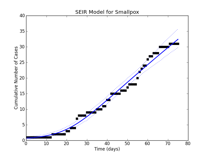
figure(1)
-
title('SEIR Model for Smallpox')
-
plot(mod.case_data, 's', mec = 'black', color = 'black')
-
plot(mod.cases.stats()['mean'], color = 'blue', linewidth = 2)
-
plot(mod.cases.stats()['95% HPD interval'], color = 'blue', linewidth = 1, linestyle = 'dotted')
-
ylabel('Cumulative Number of Cases')
-
xlabel('Time (days)')
-
savefig('fit.png')
-
-
figure(2)
-
title('Autocorrelations of unknown parameters')
-
subplot(3, 1, 1)
-
acorr(mod.beta.trace(), detrend = mlab.detrend_mean, usevlines = True)
-
text(-10, .9, 'beta')
-
subplot(3, 1, 2)
-
acorr(mod.mu.trace(), detrend = mlab.detrend_mean, usevlines = True)
-
text(-10, 1.1, 'mu')
-
subplot(3, 1, 3)
-
acorr(mod.gamma.trace(), detrend = mlab.detrend_mean, usevlines = True)
-
text(-10, .9, 'gamma')
-
savefig('autocorr.png')
The algorithm works by sampling from a Markov chain (a sequence of random vectors  such that
  depends only on
  ). It (somehow) constructs a Markov chain so that in the limit of infinitely many steps, all eventually have the same distribution
  . When solving these types of problems, the target distribution
  is the posterior distribution of the parameters given the data. The code above states that after a "burn-in period" of 5000 iterations, the chain can be considered to have converged to its stationary distribution. After this a further 55000 iterations are used to gain useful information about the parameters through Monte Carlo integration.
The most useful pieces of information to us are the moments. The components of the first moment (or the mean) are the values that we will quote as estimates of the parameters. The components of the second moment give us a kind of "error bar" - they tell us how far we can stray from the mean before the fit becomes too bad. The  moment is the horrible looking vector:
![\[<br />
\left [<br />
\begin{tabular}{c}<br />
\int\hspace{-2mm}\int\hspace{-2mm}\int\hspace{-2mm}\int\hspace{-2mm}\int\hspace{-2mm}\int\hspace{-2mm}\int_{\mathbb{R}^7} \beta^n \: g(\beta, \mu, \gamma, S_0, E_0, I_0, C_0 \: | \: A_t) \: \textup{d} \beta \textup{d} \mu \textup{d} \gamma \textup{d} S_0 \textup{d} E_0 \textup{d} I_0 \textup{d} C_0 \\<br />
\int\hspace{-2mm}\int\hspace{-2mm}\int\hspace{-2mm}\int\hspace{-2mm}\int\hspace{-2mm}\int\hspace{-2mm}\int_{\mathbb{R}^7} \mu^n \: g(\beta, \mu, \gamma, S_0, E_0, I_0, C_0 \: | \: A_t) \: \textup{d} \beta \textup{d} \mu \textup{d} \gamma \textup{d} S_0 \textup{d} E_0 \textup{d} I_0 \textup{d} C_0 \\<br />
\int\hspace{-2mm}\int\hspace{-2mm}\int\hspace{-2mm}\int\hspace{-2mm}\int\hspace{-2mm}\int\hspace{-2mm}\int_{\mathbb{R}^7} \gamma^n \: g(\beta, \mu, \gamma, S_0, E_0, I_0, C_0 \: | \: A_t) \: \textup{d} \beta \textup{d} \mu \textup{d} \gamma \textup{d} S_0 \textup{d} E_0 \textup{d} I_0 \textup{d} C_0 \\<br />
\int\hspace{-2mm}\int\hspace{-2mm}\int\hspace{-2mm}\int\hspace{-2mm}\int\hspace{-2mm}\int\hspace{-2mm}\int_{\mathbb{R}^7} S_0^n \: g(\beta, \mu, \gamma, S_0, E_0, I_0, C_0 \: | \: A_t) \: \textup{d} \beta \textup{d} \mu \textup{d} \gamma \textup{d} S_0 \textup{d} E_0 \textup{d} I_0 \textup{d} C_0 \\<br />
\int\hspace{-2mm}\int\hspace{-2mm}\int\hspace{-2mm}\int\hspace{-2mm}\int\hspace{-2mm}\int\hspace{-2mm}\int_{\mathbb{R}^7} E_0^n \: g(\beta, \mu, \gamma, S_0, E_0, I_0, C_0 \: | \: A_t) \: \textup{d} \beta \textup{d} \mu \textup{d} \gamma \textup{d} S_0 \textup{d} E_0 \textup{d} I_0 \textup{d} C_0 \\<br />
\int\hspace{-2mm}\int\hspace{-2mm}\int\hspace{-2mm}\int\hspace{-2mm}\int\hspace{-2mm}\int\hspace{-2mm}\int_{\mathbb{R}^7} I_0^n \: g(\beta, \mu, \gamma, S_0, E_0, I_0, C_0 \: | \: A_t) \: \textup{d} \beta \textup{d} \mu \textup{d} \gamma \textup{d} S_0 \textup{d} E_0 \textup{d} I_0 \textup{d} C_0 \\<br />
\int\hspace{-2mm}\int\hspace{-2mm}\int\hspace{-2mm}\int\hspace{-2mm}\int\hspace{-2mm}\int\hspace{-2mm}\int_{\mathbb{R}^7} C_0^n \: g(\beta, \mu, \gamma, S_0, E_0, I_0, C_0 \: | \: A_t) \: \textup{d} \beta \textup{d} \mu \textup{d} \gamma \textup{d} S_0 \textup{d} E_0 \textup{d} I_0 \textup{d} C_0<br />
\end{tabular}<br />
\right ]<br />
\]](/sites/default/files/tex/12ee138d6468e2c4947d7d7a6f2420de624a9e13.png) |
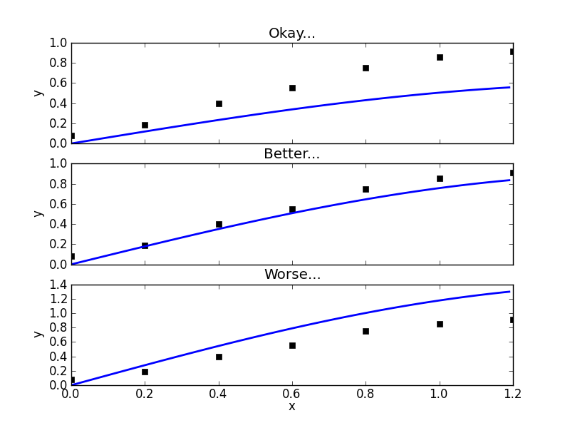
but a very close approximation to this is found if we sample from hundreds of times, raise the samples to the power and average them. The mean and the various quantiles now let us go back to the simulation of the dynamical system and plot a curve that fits the data pretty well:
Using the mean estimates, I would quote the parameters to be:
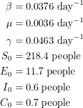 |
These estimates can only be trusted if I know that the chain has had enough iterations. How can I find this out? Well Abraham Flaxman performed two tests. One of them looks at the joint distribution of  and . Since I am simulating an SEIR model instead of an SIR model, I would want to look at the joint distribution of ,
  and . However, I don't know how to visualize this so I'll skip to the second test. This one looks at the autocorrelation. In approximating the value of , the MCMC algorithm makes many draws
  . We can therefore measure how correlated the draws are from one to the next. The formula for the autocorrelation depends on the mean
 ![$ E[\beta] $](/sites/default/files/tex/2bfcd9332ecfae3fbae4b61bb4905e608e5091b1.png) and the variance
and the variance ![$ V[\beta] $](/sites/default/files/tex/044618d22fa2cf62e3e0b80e9348912d5d792fbe.png) . As a function of the time lag
. As a function of the time lag  , the autocorrelation is:
![\[<br />
\frac{E[(\beta_{i + \Delta i} - E[\beta])(\beta_i - E[\beta])]}{V[\beta]}<br />
\]](/sites/default/files/tex/faa6b2c9d687802b6e6db7e1f6a23efd1e99136d.png) |
Up to a normalization, this is just the covariance of  and
and  which is a measure of (linear) dependence between the variables. If the samples are really independent and identically distributed as intended, the autocorrelation should vanish for every nonzero time lag. The plot that I get does this well for :
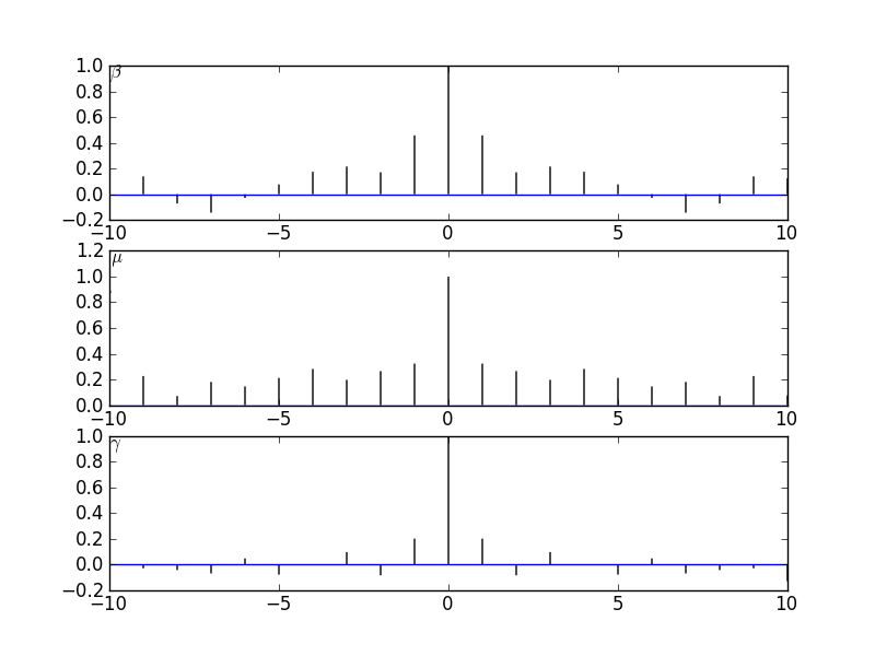
This is helped by the fact that we are "thinning" the chain by a factor of 500. The autocorrelation plots for and still do not look very sharp so if I were publishing this I'd increase the number of iterations just to be on the safe side.
This is turning out to be a long post so I will end by telling you why I think this is better than a least squares approach:
- Minimizing the sum of the squares of the residuals is only equivalent to fining the most likely set of parameters when the errors are normally distributed. Bayesian inference nicely accommodates other error models such as the Poisson distribution we have used.
- The assumption that errors are normally distributed often conflicts with a priori knowledge. For a normally distributed quantity, a two-sided confidence interval extends equally in both directions and this sometimes leads to absurdities like
 . If you know that you're measuring a mass with reasonable accuracy a normal distribution will hardly put any mass on the negative values. But if you're measuring something like the neutrino mass, you need to be doing statistics more carefully.
 - When an algorithm lets you minimize a distance, this is usually taken to be an unconstrained optimization. Since we know that the rates in an SEIR model are positive, fitting this with a least squares method would have required some annoying absolute value signs making the function harder to fit. PyMC automatically restricts the parameter space by allowing you to choose the supports of your priors.
- We did not do a fit to multiple data sets but something we could have done with other epidemiological data is fit the cumulative number of cases and the cumulative number of deaths at the same time. In a least squares fit, if thousands of people get infected but only tens of people die, this is asking for trouble. In this situation, a death value being off by 10 is worse than a case value being off by 10, but the fitter won't think so. The fitter will treat the two data sets as one concatenated data set and the normally distributed errors in a least squares model (unlike those in a Bayesian model) all need to have the same standard deviation. Unless we implement a bunch of ad-hoc scale factors, the fitter will all but ignore the time series of deaths in exchange for making the fit to the time series of cases a little bit better.
- The dotted lines that appeared in our plot showed the and percentile of the fit giving us an idea of the spread. While we can certainly get these percentiles for the regressors in a least squares fit, it is sometimes non-trivial to translate these into confidence intervals for the curve itself. Getting the percentile of the curve is not the same as evaluating the function at the percentile values of all of its parameters because some fluctuations could cancel each other out.
The only down side is that it seems easy to make PyMC crash. When I lookup the errors that I get, I keep seeing suggestions to pick better initial guesses. So the question becomes: am I good enough at doing parameter estimation in my head to write parameter estimation code that won't crash? Not yet, but I am getting better!